I used this kernel in the Kannada MNIST Competition, getting a final Private Score of 0.99040 and final Public Score of 0.98920, approximately 60th out of 1213 ( Top 5% ) on LB. Here is how this kernel implemented.
The CNN architecture is based on kernel of FWiktor. Thanks a lot to him.
CNN Architecture
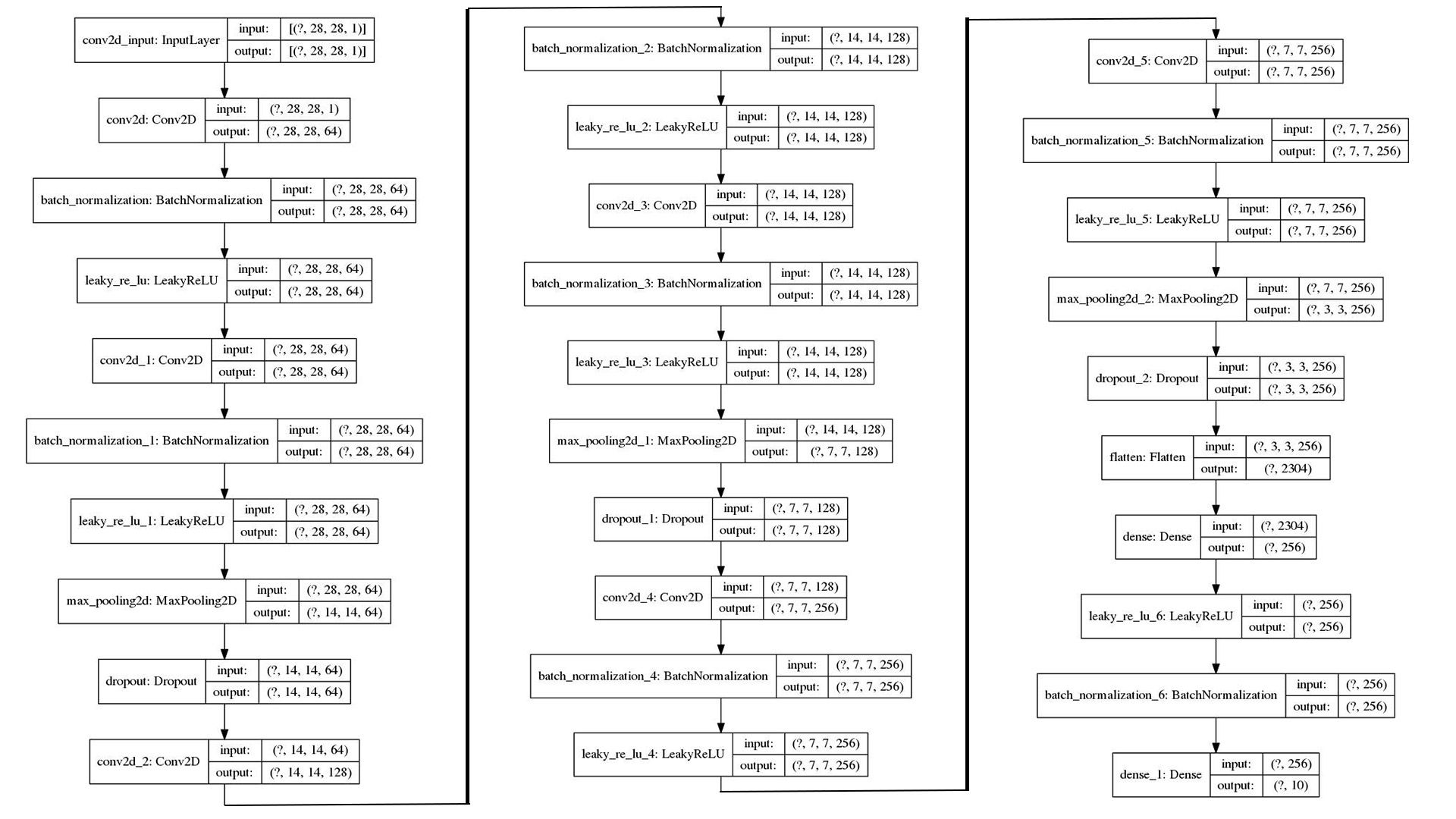
First of all, here is the architecture of FWiktor’s network:
Based on this summary, I implemented a network and reached an accuracy of 85% on val_set( Dig-MNIST.csv ). Well, the result is fairly good, but I want a even higher accuracy, something like 95% or even 99%.
In order to achieve that, I adjusted some layers of the neural network structure and added some layers as well( Will mention it later ). Here is the summary of my network:
1
2
3
4
5
6
7
8
9
10
11
12
13
14
15
16
17
18
19
20
21
22
23
24
25
26
27
28
29
30
31
32
33
34
35
36
37
38
39
40
41
42
43
44
45
46
47
48
49
50
51
52
53

----------------------------------------------------------------
        Layer (type)               Output Shape         Param #
================================================================
            Conv2d-1           [-1, 64, 28, 28]             640
       BatchNorm2d-2           [-1, 64, 28, 28]             128
         LeakyReLU-3           [-1, 64, 28, 28]               0
            Conv2d-4           [-1, 64, 28, 28]          36,928
       BatchNorm2d-5           [-1, 64, 28, 28]             128
         LeakyReLU-6           [-1, 64, 28, 28]               0
            Conv2d-7           [-1, 64, 28, 28]          36,928
       BatchNorm2d-8           [-1, 64, 28, 28]             128
         LeakyReLU-9           [-1, 64, 28, 28]               0
        MaxPool2d-10           [-1, 64, 14, 14]               0
        Dropout2d-11           [-1, 64, 14, 14]               0
           Conv2d-12          [-1, 128, 14, 14]          73,856
      BatchNorm2d-13          [-1, 128, 14, 14]             256
        LeakyReLU-14          [-1, 128, 14, 14]               0
           Conv2d-15          [-1, 128, 14, 14]         147,584
      BatchNorm2d-16          [-1, 128, 14, 14]             256
        LeakyReLU-17          [-1, 128, 14, 14]               0
           Conv2d-18          [-1, 128, 14, 14]         147,584
      BatchNorm2d-19          [-1, 128, 14, 14]             256
        LeakyReLU-20          [-1, 128, 14, 14]               0
        MaxPool2d-21            [-1, 128, 7, 7]               0
        Dropout2d-22            [-1, 128, 7, 7]               0
           Conv2d-23            [-1, 256, 7, 7]         295,168
      BatchNorm2d-24            [-1, 256, 7, 7]             512
        LeakyReLU-25            [-1, 256, 7, 7]               0
           Conv2d-26            [-1, 256, 7, 7]         590,080
      BatchNorm2d-27            [-1, 256, 7, 7]             512
        LeakyReLU-28            [-1, 256, 7, 7]               0
    GlobalAvgPool-29                  [-1, 256]               0
           Linear-30                   [-1, 32]           8,224
             ReLU-31                   [-1, 32]               0
           Linear-32                  [-1, 256]           8,448
          Sigmoid-33                  [-1, 256]               0
      Sq_Ex_Block-34            [-1, 256, 7, 7]               0
        MaxPool2d-35            [-1, 256, 3, 3]               0
        Dropout2d-36            [-1, 256, 3, 3]               0
           Linear-37                  [-1, 256]         590,080
        LeakyReLU-38                  [-1, 256]               0
      BatchNorm1d-39                  [-1, 256]             512
           Linear-40                   [-1, 10]           2,570
================================================================
Total params: 1,940,778
Trainable params: 1,940,778
Non-trainable params: 0
----------------------------------------------------------------
Input size (MB): 0.00
Forward/backward pass size (MB): 6.17
Params size (MB): 7.40
Estimated Total Size (MB): 13.58
----------------------------------------------------------------
Differences Between FWiktor’s And Mine
Two More Conv2d Layers
When I trained my model on the FWikor’s network, I found the accuracy of val_set drastically improved from 10% to 80% in a very short time, like in 5 epochs, then it continued to improve a little bit to 85% in the approximately next 40 epochs and finally remained the same no matter how much longer you trained it. I believe it is because the network is not deep enough and therefore I want a deeper network than FWictor’s. Considering the fact that MNIST dataset is somewhat straightforward and doesn’t really need more Conv2d layers to detect its high-dimensional features, I put my additional Conv2d layers to where before the first Maxpool2d layer and the second Maxpool2d layer.
Modify Layer Parameters
In the original network, the parameter for Dropout2d() is 0.5 so that in each forward call, each channel has the same probability to be zeroed out or not, which stands for a greater randomness, which is definitely good. However, in reality, there is actually a very low probability for front layers to be zeroed out in a considerably deep neural network, so I modify the parameter to 0.4 and it turns out good.
Add A Squeeze-and-Excitation Network (SE Net)
Several References About SE Net:
https://arxiv.org/abs/1709.01507
https://towardsdatascience.com/review-senet-squeeze-and-excitation-network-winner-of-ilsvrc-2017-image-classification-a887b98b2883
https://medium.com/@konpat/squeeze-and-excitation-networks-hu-et-al-2017-48e691d3fe5e
https://www.kaggle.com/c/tgs-salt-identification-challenge/discussion/65939 ( A simple SE Block implementation )
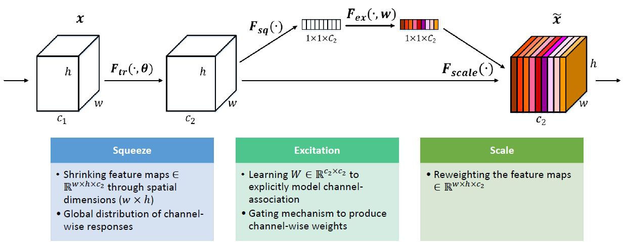
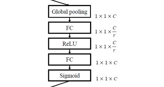
Squeeze-and-Excitation (SE) Block helps dynamically “excite” feature maps that help classification and suppress features maps that don’t help based on the patterns of global averages of feature maps.
Implementation Of The Network
Implemented by PyTorch
Import Packages
1
2
3
4
5
6
7
8
9
10
11

import numpy as np
import pandas as pd
import torch
import torch.nn as nn
from torch.utils.data import Dataset, DataLoader

import torchvision
from torchvision import transforms, datasets

from PIL import Image
import matplotlib.pyplot as plt
Implementing SE Block
1
2
3
4
5
6
7
8
9
10
11
12
13
14
15
16
17
18
19
20
21
22
23

class Sq_Ex_Block(nn.Module):
    def __init__(self, in_ch, r):
        super(Sq_Ex_Block, self).__init__()
        self.se = nn.Sequential(
            GlobalAvgPool(),
            nn.Linear(in_ch, in_ch // r),
            nn.ReLU(inplace=True),
            nn.Linear(in_ch // r, in_ch),
            nn.Sigmoid()
        )

    def forward(self, x):
        se_weight = self.se(x).unsqueeze(-1).unsqueeze(-1)
        x = x.mul(se_weight)
        return x


class GlobalAvgPool(nn.Module):
    def __init__(self):
        super(GlobalAvgPool, self).__init__()

    def forward(self, x):
        return x.view(*(x.shape[:-2]), -1).mean(-1)
Implementing Main Network
1
2
3
4
5
6
7
8
9
10
11
12
13
14
15
16
17
18
19
20
21
22
23
24
25
26
27
28
29
30
31
32
33
34
35
36
37
38
39
40
41
42
43
44
45
46
47
48
49
50
51
52
53
54
55
56
57
58
59
60
61
62
63
64
65
66
67
68
69
70
71
72
73
74
75
76
77
78
79

class KannadaNet(nn.Module):
    def __init__(self):
        super(KannadaNet, self).__init__()
        self.layer1 = nn.Sequential(
            nn.Conv2d(1, 64, 3, stride=1, padding=1),  # 28 x 28 x 1 => 28 x 28 x 64
            nn.BatchNorm2d(64, 1e-3, 1e-2),
            nn.LeakyReLU(0.1, True)
        )
        self.layer2 = nn.Sequential(
            nn.Conv2d(64, 64, 3, stride=1, padding=1),  # 28 x 28 x 64 => 28 x 28 x 64
            nn.BatchNorm2d(64, 1e-3, 1e-2),
            nn.LeakyReLU(0.1, True)
        )
        self.layer2_1 = nn.Sequential(
            nn.Conv2d(64, 64, 3, stride=1, padding=1),  # 28 x 28 x 64 => 28 x 28 x 64
            nn.BatchNorm2d(64, 1e-3, 1e-2),
            nn.LeakyReLU(0.1, True)
        )
        self.layer3 = nn.Sequential(
            nn.MaxPool2d(2, stride=2),  # 28 x 28 x 64 => 14 x 14 x 64
            nn.Dropout2d(0.4)
        )
        self.layer4 = nn.Sequential(
            nn.Conv2d(64, 128, 3, stride=1, padding=1),  # 14 x 14 x 64 => 14 x 14 x 128
            nn.BatchNorm2d(128, 1e-3, 1e-2),
            nn.LeakyReLU(0.1, True)
        )
        self.layer5 = nn.Sequential(
            nn.Conv2d(128, 128, 3, stride=1, padding=1),  # 14 x 14 x 128 => 14 x 14 x 128
            nn.BatchNorm2d(128, 1e-3, 1e-2),
            nn.LeakyReLU(0.1, True)
        )
        self.layer5_1 = nn.Sequential(
            nn.Conv2d(128, 128, 3, stride=1, padding=1),  # 14 x 14 x 128 => 14 x 14 x 128
            nn.BatchNorm2d(128, 1e-3, 1e-2),
            nn.LeakyReLU(0.1, True)
        )
        self.layer6 = nn.Sequential(
            nn.MaxPool2d(2, stride=2),  # 14 x 14 x 128 => 7 x 7 x 128
            nn.Dropout2d(0.4)
        )
        self.layer7 = nn.Sequential(
            nn.Conv2d(128, 256, 3, stride=1, padding=1),  # 7 x 7 x 128 => 7 x 7 x 256
            nn.BatchNorm2d(256, 1e-3, 1e-2),
            nn.LeakyReLU(0.1, True)
        )
        self.layer8 = nn.Sequential(
            nn.Conv2d(256, 256, 3, stride=1, padding=1),  # 7 x 7 x 256 => 7 x 7 x 256
            nn.BatchNorm2d(256, 1e-3, 1e-2),
            nn.LeakyReLU(0.1, True)
        )
        self.layer9 = nn.Sequential(
            Sq_Ex_Block(in_ch=256, r=8),
            nn.MaxPool2d(2, stride=2),  # 7 x 7 x 256 => 3 x 3 x 256
            nn.Dropout2d(0.4)
        )
        self.dense = nn.Sequential(
            nn.Linear(2304, 256),
            nn.LeakyReLU(0.1, True),
            nn.BatchNorm1d(256, 1e-3, 1e-2)
        )
        self.fc = nn.Linear(256, 10)

    def forward(self, x):
        x = self.layer1(x)
        x = self.layer2(x)
        x = self.layer2_1(x)
        x = self.layer3(x)
        x = self.layer4(x)
        x = self.layer5(x)
        x = self.layer5_1(x)
        x = self.layer6(x)
        x = self.layer7(x)
        x = self.layer8(x)
        x = self.layer9(x)
        x = x.view(-1, 3 * 3 * 256)
        x = self.dense(x)
        x = self.fc(x)
        return x
Some Other Tips On Kannaba MNIST
Data Augmentation
Data augmentation was performed with these parameters:
1
2
3
4

train_transform = transforms.Compose([
    transforms.RandomAffine(10, (0.25, 0.25), (0.8, 1.2), 5),
    transforms.ToTensor()
])
I Use RMSProp Optimizer
1

optimizer = torch.optim.RMSprop(kannada_net.parameters(), lr=1e-3, alpha=0.9)
I Use ReduceLROnPlateau Scheduler
1

scheduler = torch.optim.lr_scheduler.ReduceLROnPlateau(optimizer, factor=0.5, verbose=True)
Save The Model That Has The Best Accuracy
1
2
3
4
5
6
7
8
9
10
11
12

max_acc = 0
best_model_dict = None

train(…)
val(…)

if acc > max_acc:
    max_acc = acc
    best_model_dict = kannada_net.state_dict()

# Predicting
kannada_net.load_state_dict(best_model_dict)
Automatically Quit Training To Save Time
1
2
3

if optimizer.param_groups[0]['lr'] < 5e-5:
    print("Learning Rate is Smaller than 0.00005, Stoping Trainning")
    break
Source Code
Thanks for reading and please leave an UPVODE if you find it useful.
本文作者 Auther:Soptq
本文链接 Link: https://soptq.me/2020/01/21/kannada_kernel/
版权声明 Copyright: 本博客所有文章除特别声明外,均采用 CC BY-NC-SA 4.0 许可协议。转载请注明出处。 Content on this site is licensed under the CC BY-NC-SA 4.0 license agreement unless otherwise noted. Attribution required.
发现存在错别字或者事实错误?请麻烦您点击 这里 汇报。谢谢您!


